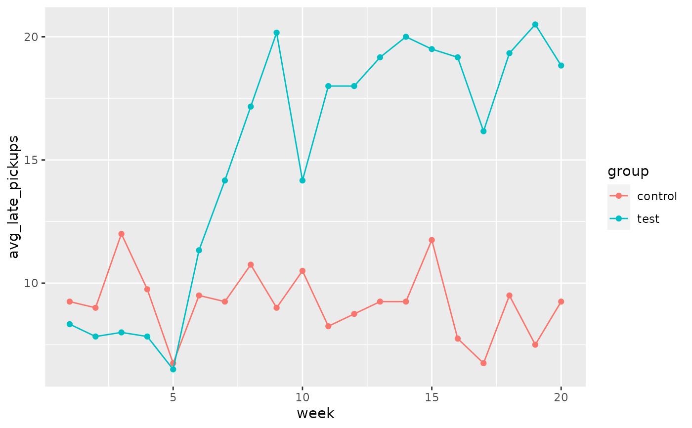
Researchers tested the deterrence hypothesis which predicts that the introduction of a penalty will reduce the occurrence of the behavior subject to the fine, with the condition that the fine leaves everything else unchanged by instituting a fine for late pickup at daycare centers. For this study, they worked with 10 volunteer daycare centers that did not originally impose a fine to parents for picking up their kids late. They randomly selected 6 of these daycare centers and instituted a monetary fine (of a considerable amount) for picking up children late and then removed it. In the remaining 4 daycare centers no fine was introduced. The study period was divided into four: before the fine (weeks 1–4), the first 4 weeks with the fine (weeks 5-8), the entire period with the fine (weeks 5–16), and the after fine period (weeks 17-20). Throughout the study, the number of kids who were picked up late was recorded each week for each daycare. The study found that the number of late-coming parents increased significantly when the fine was introduced, and no reduction occurred after the fine was removed.
Format
A data frame with 200 observations on the following 7 variables.
- center
Daycare center id.
- group
Study group:
test(fine instituted) orcontrol(no fine).- children
Number of children at daycare center.
- week
Week of study.
- late_pickups
Number of late pickups for a given week and daycare center.
- study_period_4
Period of study, divided into 4 periods:
before fine,first 4 weeks with fine,last 8 weeks with fine,after fine- study_period_3
Period of study, divided into 4 periods:
before fine,with fine,after fine
Source
Gneezy, Uri, and Aldo Rustichini. "A fine is a price." The Journal of Legal Studies 29, no. 1 (2000): 1-17.
Examples
library(dplyr)
library(tidyr)
library(ggplot2)

# The following tables roughly match results presented in Table 2 of the source article
# The results are only off by rounding for some of the weeks
daycare_fines |>
  group_by(center, study_period_4) |>
  summarise(avg_late_pickups = mean(late_pickups), .groups = "drop") |>
  pivot_wider(names_from = study_period_4, values_from = avg_late_pickups)
#> # A tibble: 10 × 5
#>    center `before fine` `first 4 weeks with fine` `last 8 weeks with fine`
#>     <int>         <dbl>                     <dbl>                    <dbl>
#>  1      1          7.25                       9.5                    14.1
#>  2      2          5.25                       9                      13.9
#>  3      3          8.5                       10.2                    20.1
#>  4      4          9                         15                      21.2
#>  5      5         11.8                       20                      27
#>  6      6          6.25                      10                      14.8
#>  7      7          8.75                       8                       6.88
#>  8      8         13.2                       10.5                    11.1
#>  9      9          4.75                       5.5                     5.62
#> 10     10         13.2                       12.2                    13.6
#> # ℹ 1 more variable: `after fine` <dbl>

daycare_fines |>
  group_by(center, study_period_3) |>
  summarise(avg_late_pickups = mean(late_pickups), .groups = "drop") |>
  pivot_wider(names_from = study_period_3, values_from = avg_late_pickups)
#> # A tibble: 10 × 4
#>    center `before fine` `with fine` `after fine`
#>     <int>         <dbl>       <dbl>        <dbl>
#>  1      1          7.25       12.6         15.2
#>  2      2          5.25       12.2         13.2
#>  3      3          8.5        16.8         22
#>  4      4          9          19.2         20.2
#>  5      5         11.8        24.7         29.5
#>  6      6          6.25       13.2         12
#>  7      7          8.75        7.25         6.75
#>  8      8         13.2        10.9          9.25
#>  9      9          4.75        5.58         4.75
#> 10     10         13.2        13.2         12.2

# The following plot matches Figure 1 of the source article
daycare_fines |>
  group_by(week, group) |>
  summarise(avg_late_pickups = mean(late_pickups), .groups = "drop") |>
  ggplot(aes(x = week, y = avg_late_pickups, group = group, color = group)) +
  geom_point() +
  geom_line()