American Community Survey, 2012 — acs12 • openintro

Results from the US Census American Community Survey, 2012.

Usage

acs12

Format

A data frame with 2000 observations on the following 13 variables.

income: Annual income.
employment: Employment status.
hrs_work: Hours worked per week.
race: Race.
age: Age, in years.
gender: Gender.
citizen: Whether the person is a U.S. citizen.
time_to_work: Travel time to work, in minutes.
lang: Language spoken at home.
married: Whether the person is married.
edu: Education level.
disability: Whether the person is disabled.
birth_qrtr: The quarter of the year that the person was born, e.g. Jan thru Mar.

Source

https://www.census.gov/programs-surveys/acs

Examples


library(dplyr)
#> 
#> Attaching package: ‘dplyr’
#> The following objects are masked from ‘package:stats’:
#> 
#>     filter, lag
#> The following objects are masked from ‘package:base’:
#> 
#>     intersect, setdiff, setequal, union
library(ggplot2)
library(broom)

# employed only
acs12_emp <- acs12 %>%
  filter(
    age >= 30, age <= 60,
    employment == "employed",
    income > 0
  )

# linear model
ggplot(acs12_emp, mapping = aes(x = age, y = income)) +
  geom_point() +
  geom_smooth(method = "lm")
#> `geom_smooth()` using formula = 'y ~ x'


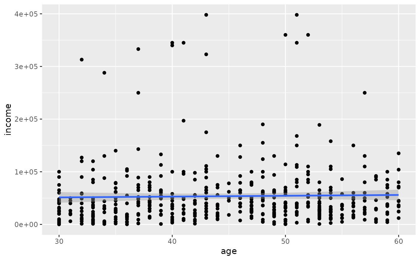lm(income ~ age, data = acs12_emp) %>%
  tidy()
#> # A tibble: 2 × 5
#>   term        estimate std.error statistic  p.value
#>   <chr>          <dbl>     <dbl>     <dbl>    <dbl>
#> 1 (Intercept)   46579.    13600.     3.43  0.000664
#> 2 age             156.      297.     0.524 0.600   

# log-transormed model
ggplot(acs12_emp, mapping = aes(x = age, y = log(income))) +
  geom_point() +
  geom_smooth(method = "lm")
#> `geom_smooth()` using formula = 'y ~ x'


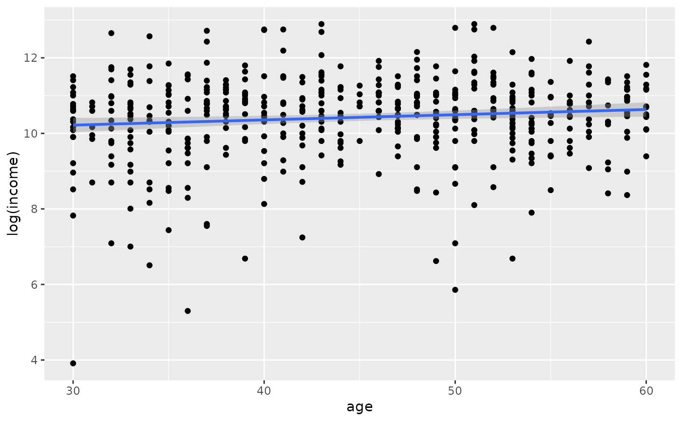lm(log(income) ~ age, data = acs12_emp) %>%
  tidy()
#> # A tibble: 2 × 5
#>   term        estimate std.error statistic   p.value
#>   <chr>          <dbl>     <dbl>     <dbl>     <dbl>
#> 1 (Intercept)   9.81     0.256       38.3  2.47e-152
#> 2 age           0.0138   0.00559      2.46 1.41e-  2