SAT and GPA data

SAT and GPA data for 1000 students at an unnamed college.

Usage

satgpa

Format

A data frame with 1000 observations on the following 6 variables.

sex

Gender of the student.

sat_v

Verbal SAT percentile.

sat_m

Math SAT percentile.

sat_sum

Total of verbal and math SAT percentiles.

hs_gpa

High school grade point average.

fy_gpa

First year (college) grade point average.

Source

Educational Testing Service originally collected the data.

References

https://chance.dartmouth.edu/course/Syllabi/Princeton96/ETSValidation.html

Examples

library(ggplot2)
library(broom)

# Verbal scores
ggplot(satgpa, aes(x = sat_v, fy_gpa)) +
  geom_point() +
  geom_smooth(method = "lm") +
  labs(
    x = "Verbal SAT percentile",
    y = "First year (college) grade point average"
  )
#> `geom_smooth()` using formula = 'y ~ x'


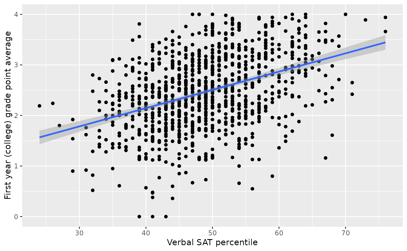mod <- lm(fy_gpa ~ sat_v, data = satgpa)
tidy(mod)
#> # A tibble: 2 × 5
#>   term        estimate std.error statistic  p.value
#>   <chr>          <dbl>     <dbl>     <dbl>    <dbl>
#> 1 (Intercept)   0.701    0.129        5.41 7.71e- 8
#> 2 sat_v         0.0361   0.00261     13.8  5.30e-40

# Math scores
ggplot(satgpa, aes(x = sat_m, fy_gpa)) +
  geom_point() +
  geom_smooth(method = "lm") +
  labs(
    x = "Math SAT percentile",
    y = "First year (college) grade point average"
  )
#> `geom_smooth()` using formula = 'y ~ x'


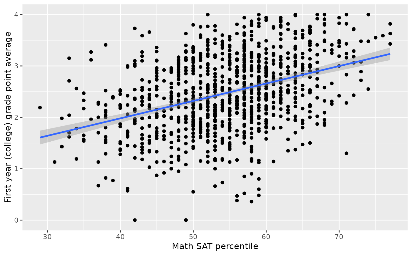mod <- lm(fy_gpa ~ sat_m, data = satgpa)
tidy(mod)
#> # A tibble: 2 × 5
#>   term        estimate std.error statistic  p.value
#>   <chr>          <dbl>     <dbl>     <dbl>    <dbl>
#> 1 (Intercept)   0.622    0.141        4.42 1.12e- 5
#> 2 sat_m         0.0339   0.00256     13.3  4.24e-37